Waterfall

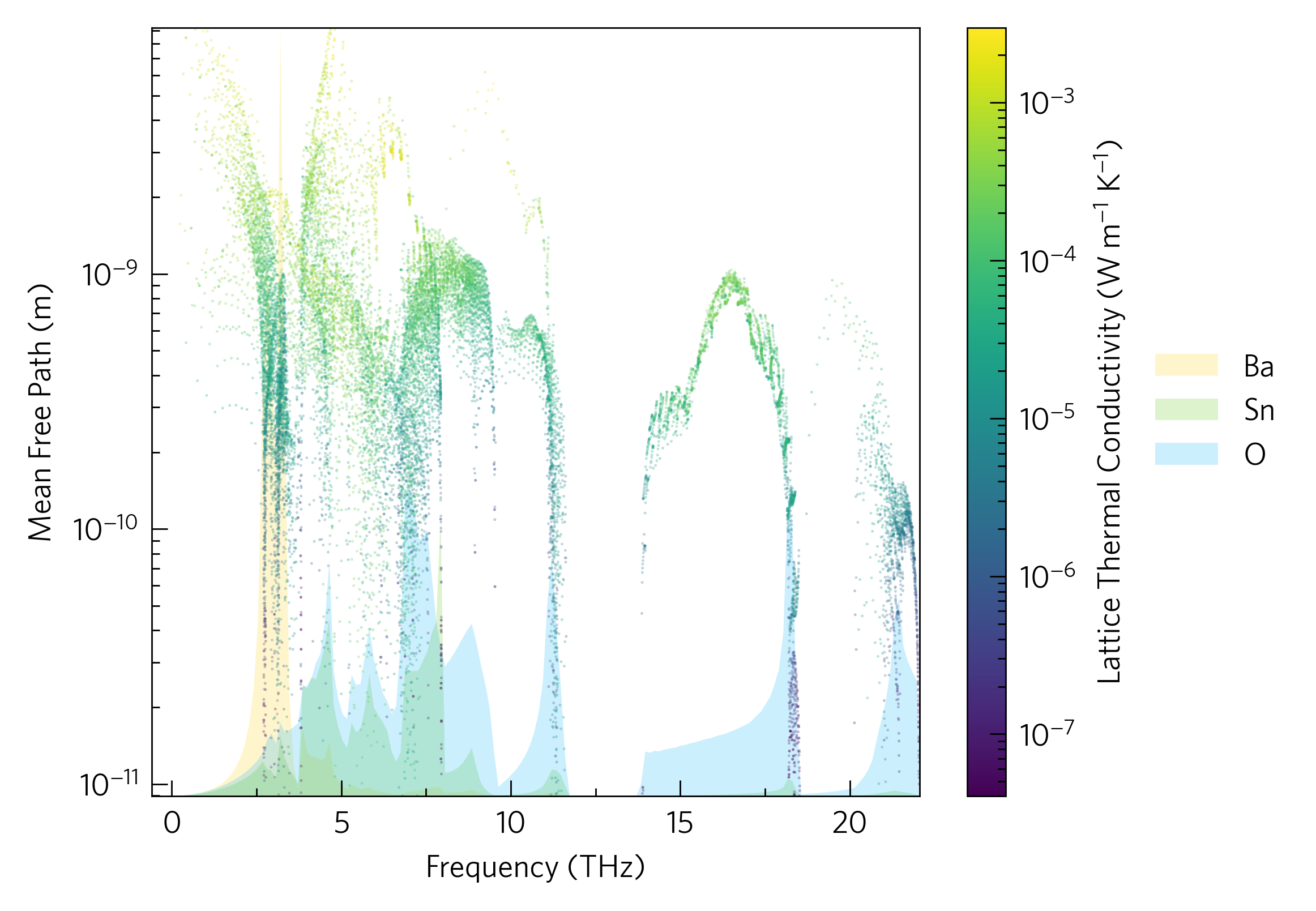
This shows a plot of mean free path against frequency with lattice thermal conductivity projected on the colour axis, as well as a density of states (DoS). It shows the connections between phonon scattering and the constituent elements, for example there seems to be a big drop in phonon mean free path in the frequencies with high amounts of Ba character.

While plots cannot be layered at the command line like this, the waterfall section can be plotted with:

tp plot waterfall ../data/basno3/kappa-m363636.hdf5 -y mfp --projected kappa

And in python:

#!/usr/bin/env python3

import tp

kfile = '../data/basno3/kappa-m363636.hdf5'
dfile = '../data/basno3/projected_dos.dat'
poscar = '../data/basno3/POSCAR'

# <ignore>
from os import path
if not path.isfile(kfile) or (path.getsize(kfile) < 1024*1024*100):
    raise Exception('File not found, please use get-data.sh in the folder above.')
# </ignore>

direction = 'avg'
temperature = 300
waterfall = 'mean_free_path'
projected = 'mode_kappa'
# Note for cumkappa and waterfall plots, mode_kappa and not kappa is required
quantities = ['waterfall', waterfall, projected]
# waterfall is an alias for frequency

colours = {'Ba': '#ffcf06',
           'Sn': '#59c605',
           'O':  '#00b1f7'}
colour = 'viridis'

# Axes
fig, ax, add_legend = tp.axes.small.one_colourbar()

# Load
data = tp.data.load.phono3py(kfile, quantities=quantities)
dos = tp.data.load.phonopy_dos(dfile, poscar=poscar)

# Add
tp.plot.frequency.format_waterfall(ax, data, waterfall, direction=direction,
                                   temperature=temperature)
tp.plot.frequency.add_dos(ax, dos, colour=colours, scale=True, main=False,
                          alpha=0.6, line=False)
cbar = tp.plot.frequency.add_projected_waterfall(ax, data, waterfall,
                                                 projected, colour=colour,
                                                 temperature=temperature,
                                                 direction=direction)
add_legend()

# Save

fig.savefig('waterfall.pdf')
fig.savefig('waterfall.png')

This example highlights a complication: in order for the waterfall to be on top of the DoS, so as not to obscure the projected colour, an additional command, format_waterfall, must be used so the DoS can be scaled correctly but plotted first (line 36-37).

Replacing add_projected_waterfall with simply add_waterfall removes the projection, and colours it with a single colour or by band index as you prefer. This is achieved by removing the --projected tag at the command line.

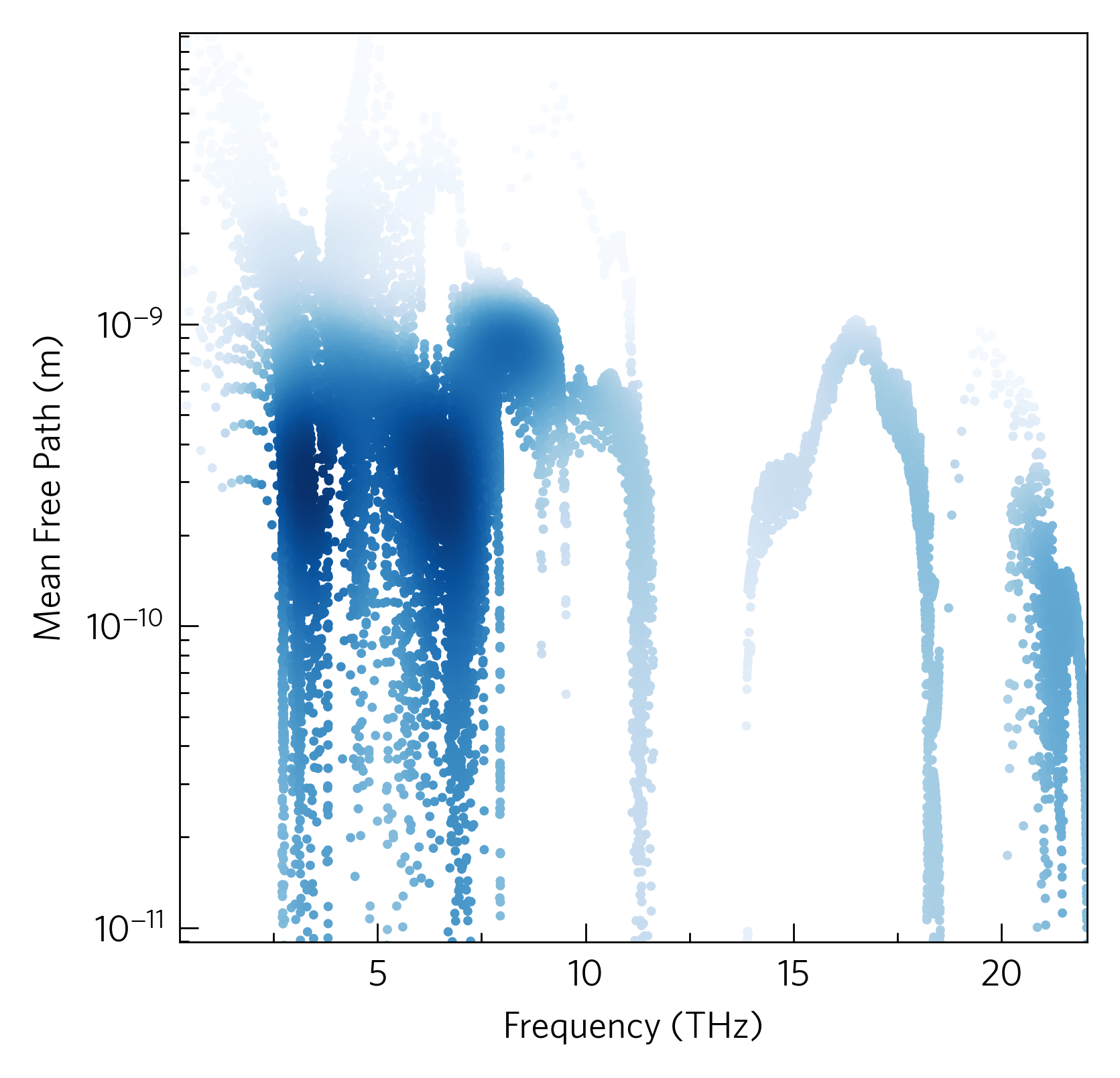
This is an alternative of the waterfall plot, where the colour darkness shows the density of the points, which is often clearer than just adjusting the alpha parameter on the regular waterfall plot.

It can be plotted at the command line with:

tp plot waterfall ../data/basno3/kappa-m363636.hdf5 -y mfp --projected density -c Blues

Or in python with:

#!/usr/bin/env python3

import tp

kfile = '../data/basno3/kappa-m363636.hdf5'
# <ignore>
from os import path
if not path.isfile(kfile) or (path.getsize(kfile) < 1024*1024*100):
    raise Exception('File not found, please use get-data.sh in the folder above.')
# </ignore>

direction = 'avg'
temperature = 300
waterfall = 'mean_free_path'
quantities = ['waterfall', waterfall]
# waterfall is an alias for frequency

colour = 'Blues'

# Axes
fig, ax, add_legend = tp.axes.small.one()

# Load
data = tp.data.load.phono3py(kfile, quantities=quantities)

# Add
tp.plot.frequency.add_density(ax, data, waterfall, colour=colour,
                              temperature=temperature, direction=direction)

# Save

fig.savefig('density.pdf')
fig.savefig('density.png')