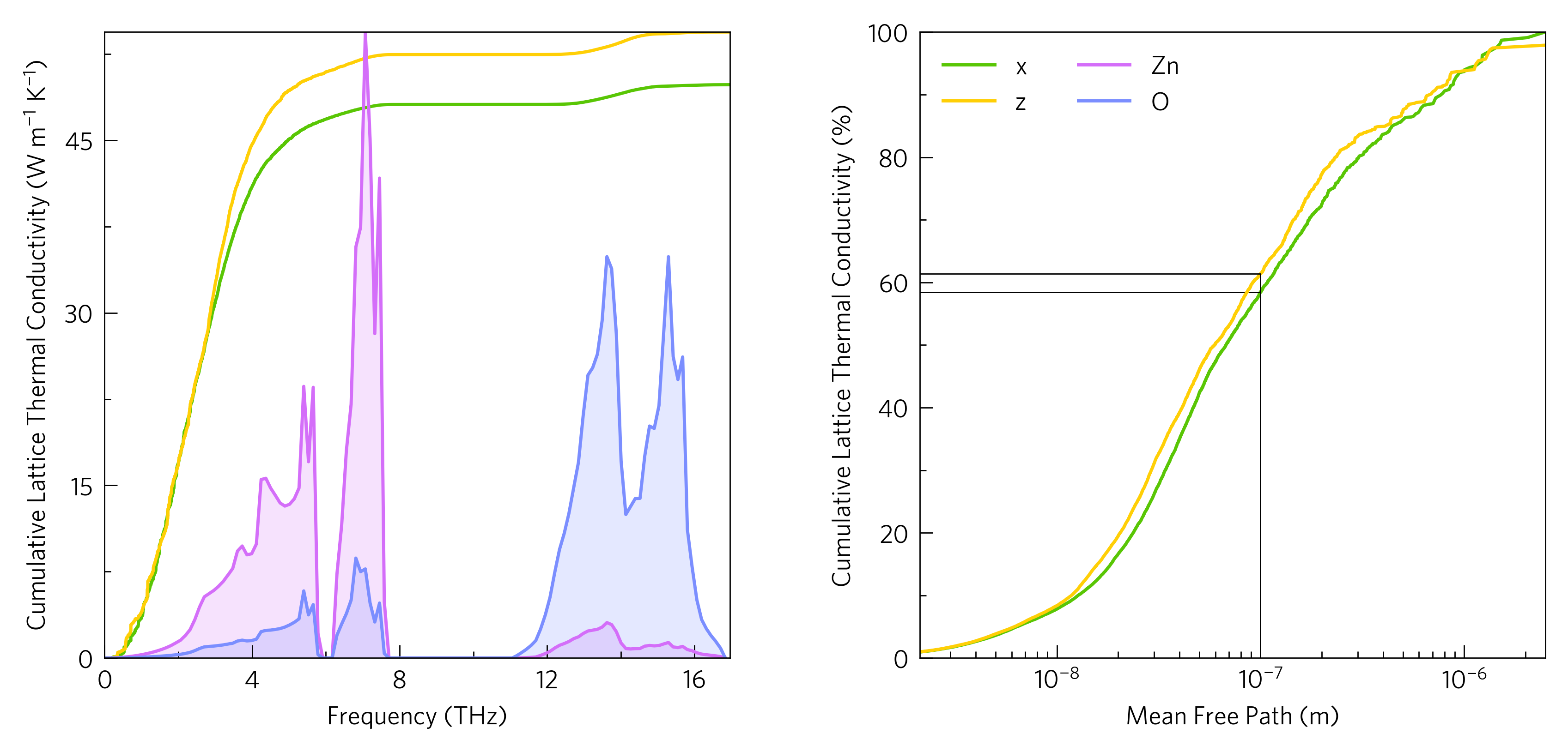
Cumulative Lattice Thermal Conductivity

This shows two plots of cumulative lattice thermal conductivity. The first one is against frequency, and particularly in conjunction with a density of states (DoS) or a phonon band structure, this can show the relative contributions of the constituent atoms to the lattice thermal conductivity. The second is against mean free path, and can be used to approximate the effect of nanostructuring, for which reason the ability to add markers has been included, e.g. here you can see nanostructuring to 100 nanometers may reduce the lattice thermal conductivity by around 40 %.

The right plot can be plotted at the command line with:

tp plot cumkappa ../data/zno/kappa-m404021.hdf5 --mfp --percent -d x -d y -c '#59c605' -c '#ffcf06' --nofill --xmarkers 1e-7 -l x -l y --location in

And while the layering of the DoS plot is not yet supported at the command line, the cumkappa part of the left graph can be plotted by removing --mfp --percent --xmarkers 1e-7 from the above.

The python version is as follows:

#!/usr/bin/env python3

import tp

kappafile = '../data/zno/kappa-m404021.hdf5'
temperature = 300
direction = ['x', 'z']
quantities = 'frequency mode_kappa mfp'
# Note for cumkappa and waterfall plots, mode_kappa and not kappa is required

# You can ignore this section
from os import path
if not path.isfile(kappafile) or (path.getsize(kappafile) < 1024*1024*100):
    raise Exception('File not found, please use get-data.sh in the folder above.')
# End ignore

dosfile = '../data/zno/projected_dos.dat'
poscar = '../data/zno/POSCAR'

colour = ['#59c605', '#ffcf06']
colours = {'Zn': '#d46ef9',
           'O':  '#7b8eff'}
# Axes
fig, ax, add_legend = tp.axes.small.two_h()

# Load
data = tp.data.load.phono3py(kappafile, quantities=quantities)
dos = tp.data.load.phonopy_dos(dosfile, poscar=poscar)

# Add
tp.plot.frequency.add_cum_kappa(ax[0], data, temperature=temperature,
                                direction=direction, colour=colour)
tp.plot.mfp.add_cum_kappa(ax[1], data, temperature=temperature, scale=True,
                          direction=direction, colour=colour, xmarkers=1e-7)
tp.plot.frequency.add_dos(ax[0], dos, colour=colours, scale=True, main=False)

add_legend(location=2, ncol=2)

# Save
fig.savefig('cumkappa.pdf')
fig.savefig('cumkappa.png')

In order to combine frequency plots, there are two important tags, main, which controls the setting of axis limits and labels, and shouls be False for all but the main plot; and scale, which scales the data to the axes, allowing diverse plots to share :rainbow: (line 35). An alternative usage of these is if both are True, it scales to percent (line 33). This is done with the --percent tag at the command line.

The markers are added with the xmarkers tag (line 34), and have a counterpart, ymarkers.

This also demonstrates use of the add_legend function supplied with tp.axes functions (line 37), which combines the legends of all plots and places itself in one of several pre-programmed position, which you can select with the location argument. Numbers will place the legend in one of the axes with loc='best', and there are also several descriptive positions, such as above and right. It also accepts most ax.legend arguements such as title and ncol. If you want to use custom handles and labels in a multi-axes figure (including DoS axes), you must specify custom=True.