Heatmaps

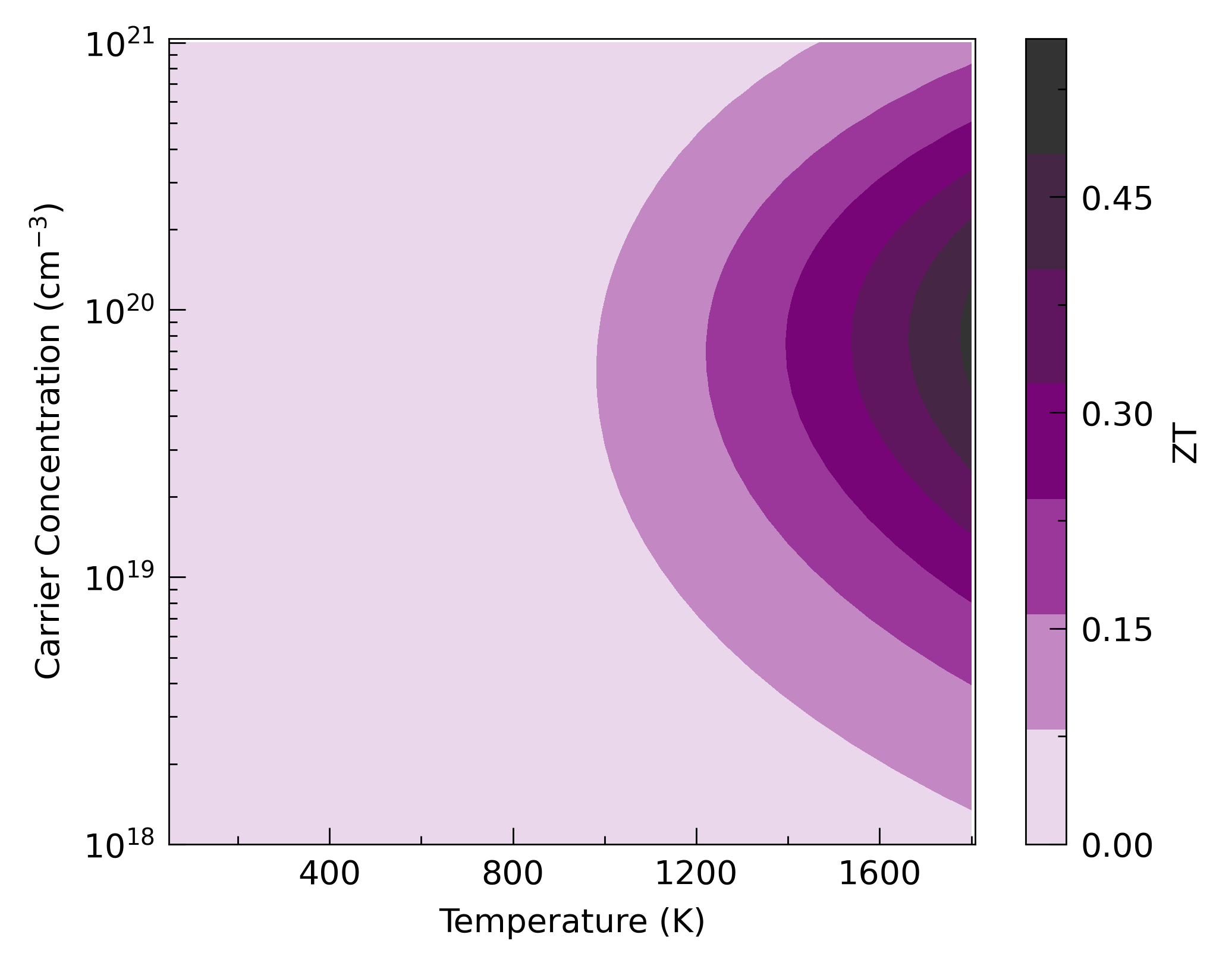
This shows the classic ZT against carrier concentration and temperature heatmap. This can be plotted at the command line with:

tp plot ztmap ../data/zno/boltztrap.hdf5 -k ../data/zno/kappa-m404021.hdf5 -c '#800080' -d x --discrete

and in python with:

#!/usr/bin/env python3

from os import path
import tp

bfile = '../data/zno/boltztrap.hdf5'
kfile = '../data/zno/kappa-m404021.hdf5'
if not path.isfile(kfile) or (path.getsize(kfile) < 1024*1024*100):
    raise Exception('File not found, please use get-data.sh in the folder above.')

direction = 'x'
colour = '#800080'

# Axes
fig, ax, add_legend = tp.axes.small.one_colourbar()

# Load
adata = tp.data.load.boltztrap(bfile)
kdata = tp.data.load.phono3py(kfile)

# Add
tp.plot.heatmap.add_ztmap(ax, adata, kdata, direction=direction, colour=colour,
                          discrete=True)

# Save
fig.savefig('ztmap.pdf')
fig.savefig('ztmap.png')

This uses the tp.plot.heatmap.add_ztmap function (line 22), which calculates the ZT and sets the axes labels. All the other functionality is wrapped within the tp.plot.heatmap.add_heatmap function, which enhances pcolourmesh in ways such as automatic rescaling of axes to represent all data, automatic extension of colourbars if applicable and custom colourmaps, which are generated dynamically with the input of a single colour, in hex, rgb (array) or named colour format. In this case, the tp.plot.colour.uniform colourmap generator has been used, which calculates a uniform colourmap between white, a supplied highlight colour and black, or three colours of your choosing. There are several other heatmap functions in ThermoParser, including the equivalent for power factor, add_pfmap, and those below…

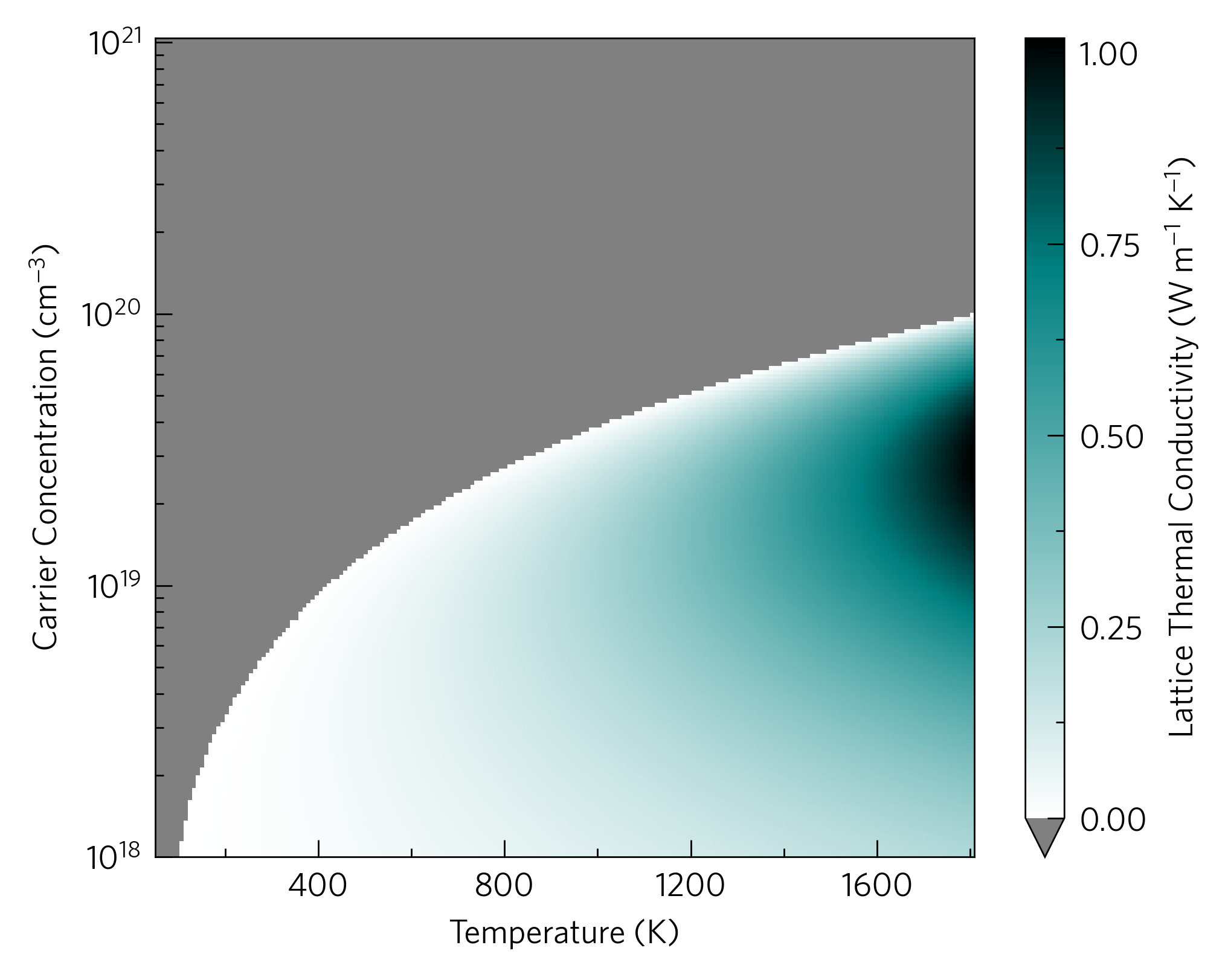
It is possible to plot a ztmap without lattice thermal conductivity data, in which case it will be set to 1 W m^-1 K^-1, which will be recorded in data['meta']['kappa_source'] (other numbers can be specified). The above is an alternative, which plots the lattice thermal conductivity required to reach a specified ZT. We hope this is a valuable tool to help decide wether to run expensive lattice thermal conductivity calculations on a material. The CLI is:

tp plot kappa-target ../data/zno/boltztrap.hdf5 -c '#008080' -d x

and python:

#!/usr/bin/env python3

import tp

f = '../data/zno/boltztrap.hdf5'
target = 2
direction = 'x'

colour = tp.plot.colour.uniform('#008080')

# Axes
fig, ax, _ = tp.axes.small.one_colourbar()

# Load
data = tp.data.load.boltztrap(f)

# Add
tp.plot.heatmap.add_kappa_target(ax, data, zt=target, colour=colour,
                                 direction=direction)

# Save
fig.savefig('kappa-target.pdf')
fig.savefig('kappa-target.png')

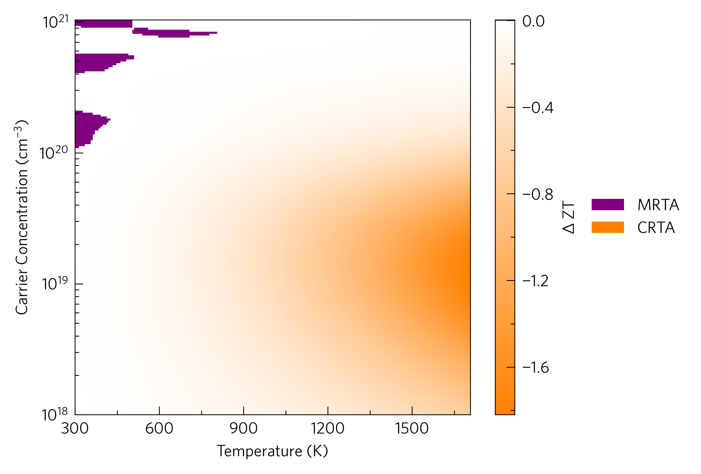
The final heatmap is the ztdiff, which compares the ZTs of two materials at a range of carrier concentrations and temperatures. This can be done with any two materials, from completely different to the same material under different conditions (e.g. different degrees of nanostructuring), although this method is most appropriate for closely related materials with similar dopabilities. Here we compare the momentum relaxation time approximation via AMSET with the constant relaxation approximation via BoltzTraP. At the command line:

tp plot ztdiff ../data/basno3/transport_75x75x75.json  ../data/basno3/boltztrap.hdf5 -k ../data/basno3/kappa-m363636.hdf5 ../data/basno3/kappa-m363636.hdf5 -l MRTA -l CRTA

and in python:

#!/usr/bin/env python3

from os import path
import tp

efiles = ['../data/basno3/transport_75x75x75.json',
          '../data/basno3/boltztrap.hdf5']
kfile = '../data/basno3/kappa-m363636.hdf5'
label = ['MRTA', 'CRTA']
if not path.isfile(kfile) or (path.getsize(kfile) < 1024*1024*100):
    raise Exception('File not found, please use get-data.sh in the folder above.')

# Axes
fig, ax, add_legend = tp.axes.small.one_colourbar()

# Load
adata = [tp.data.load.amset(efiles[0]),
         tp.data.load.boltztrap(efiles[1])]
kdata = tp.data.load.phono3py(kfile)

# Add
_, h, l = tp.plot.heatmap.add_ztdiff(ax, *adata, kdata, kdata, label1=label[0],
                                     label2=label[1])

add_legend(handles=h, labels=l)

# Save
fig.savefig('ztdiff.pdf')
fig.savefig('ztdiff.png')

Note how list comprehensions and expansions (lines 19-20 and 23 respectively) can make the script tidier. On top of the colourbar (here thrown away with _), this function returns the handles and labels which must be put into the legend manually if you want it. If you are using an axes template with multiple sets of axes, the custom argument must be used in add_legend to enable manual manipulation of the handles and labels. add_ztdiff and its power factor equivalent, add_pfdiff, also make sure the colour scale is centred on zero (i.e. where both are equal).

Some users may find adding contours with the contours argument or making the colour scale discrete with the discrete argument more legible or informative.