Disordered NaBiS2 with atomic/orbital projections & DOS plotting#
Note
The files needed for reproducing this example are provided in the examples/NaBiS2 folder.
In this example, we unfold the bands from a 80-atom special-quasirandom (SQS) supercell of NaBiS2, where the Na and Bi cations are quasi-randomly distributed, in order to simulate randomised cation disorder in the material.
These results were published in Y. T. Huang & S. R. Kavanagh et al. 2022 [1], and an early version of easyunfold was
used for the similar AgBiS\(_2\) in Y. Wang & S. R. Kavanagh et al. 2022 [2], with these plots demonstrating the key
differences in electronic structure and thus photovoltaic performance between these two materials.
Standard Unfolded Band Structure#
We have previously calculated the easyunfold.json file from the calculation using easyunfold calculate WAVECAR.
Using easyunfold unfold plot --intensity 2, we obtain the following unfolded band structure:
Unfolded band structure of \(\ce{NaBiS2}\)#
Visualisation Customisation: Colour map and intensity scaling#
The band structure above is nice, but we can make the plot a little clearer by adjusting some of the parameters like
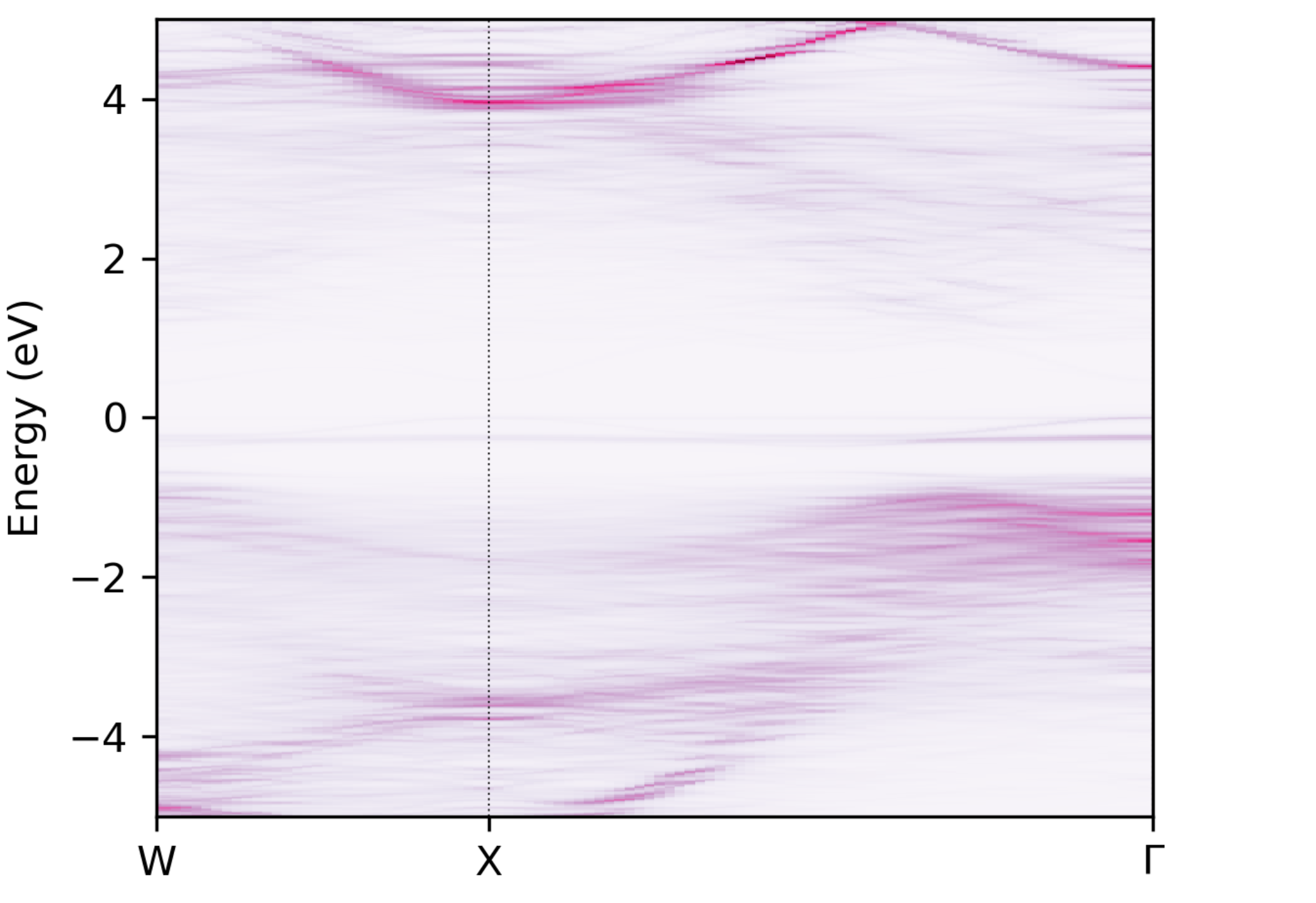
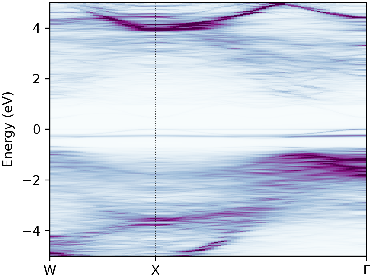
the intensity scaling (via --intensity) and the colour map (via --cmap). Below we set --intensity 2.5 to
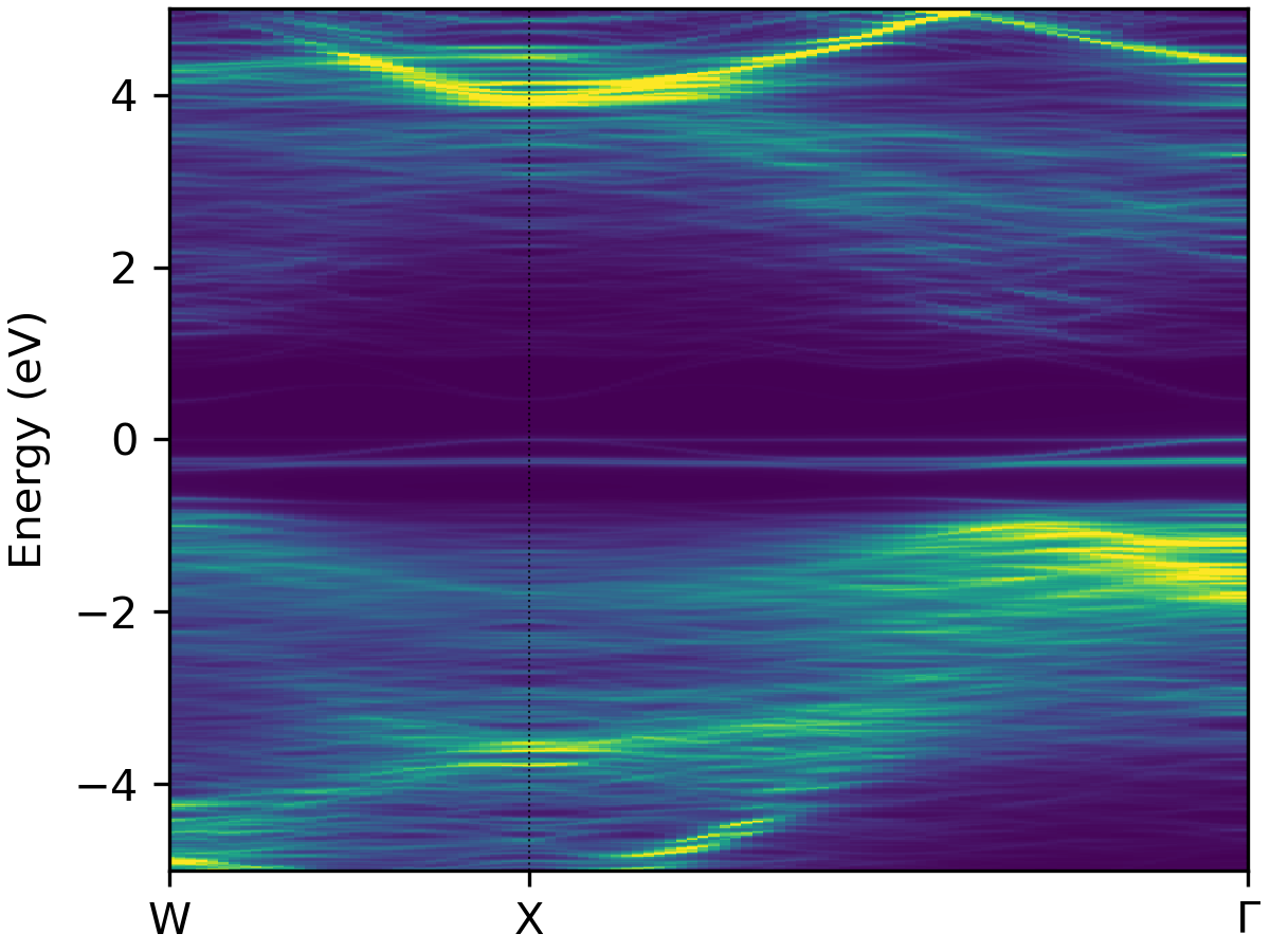
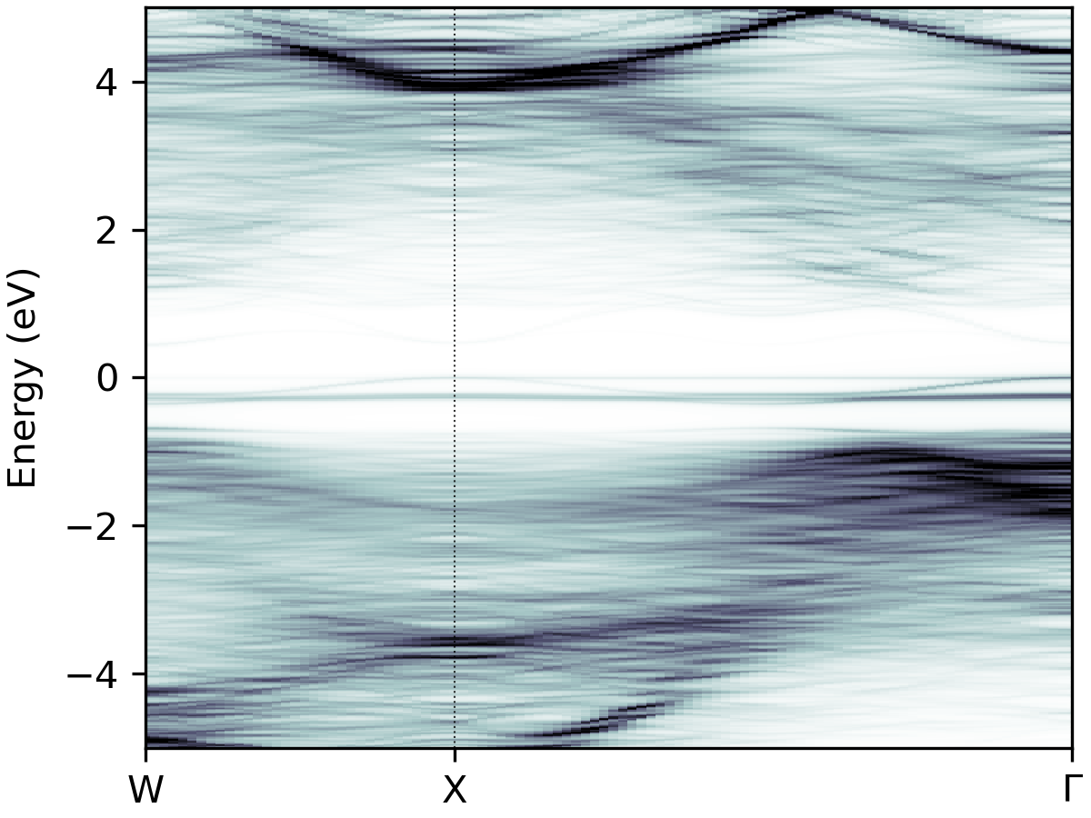
increase the colourmap intensity, and try BuPu, viridis and bone_r from left to right below:
easyunfold unfold plot --intensity 2.5 --cmap "BuPu"
easyunfold unfold plot --intensity 2.5 --cmap "viridis"
easyunfold unfold plot --intensity 2.5 --cmap "bone_r"
BuPu |
viridis |
bone_r |
|---|---|---|
|
|
|
Unfolded Band Structure with Density of States (DOS)#
We can plot the electronic density of states (DOS) alongside the unfolded band structure using the --dos option to
provide the vasprun.xml(.gz) file from our supercell calculation:
easyunfold unfold plot --intensity 2 --dos vasprun.xml.gz --zero-line --dos-label DOS --gaussian 0.1
Here we’ve used some other plot options to customise the DOS plot; see the help message with
easyunfold unfold plot -h for more info on this.
Unfolded band structure of NaBiS2 alongside the electronic density of states (DOS)#
Note
For unfolded band structures calculated with (semi-)local DFT (LDA/GGA), you should not use the vasprun.xml(.gz)
from the band structure calculation (which uses a non-uniform k-point mesh, thus giving an unrepresentative DOS
output), but rather the preceding self-consistent calculation (used to obtain the CHGCAR for the LDA/GGA DOS
calculation), or a separate DOS calculation.
Tip
To use the DOS plotting functionality of easyunfold, the sumo package must be installed. This is currently an
optional dependency for easyunfold (to avoid strict requirements and pymatgen dependencies), but can be installed
with pip install sumo.
Atom-Projected Unfolded Band Structure#
We can also plot the unfolded band structure with atomic projections, which is useful for understanding the electronic
structure of the material. In this case, we are curious as to which atoms are contributing to the band edges, and so
the atomic projections will be useful. For this, we need the PROCAR(.gz) output from VASP with the atomic and orbital
projection information, and so LORBIT should be set to 11, 12, 13 or 14 in the INCAR for the supercell
calculation.
When plotting the unfolded band, the plot-projections subcommand is used with the --procar <PROCAR> and
--atoms options:
easyunfold unfold plot-projections --atoms="Na,Bi,S" --intensity 3 --combined
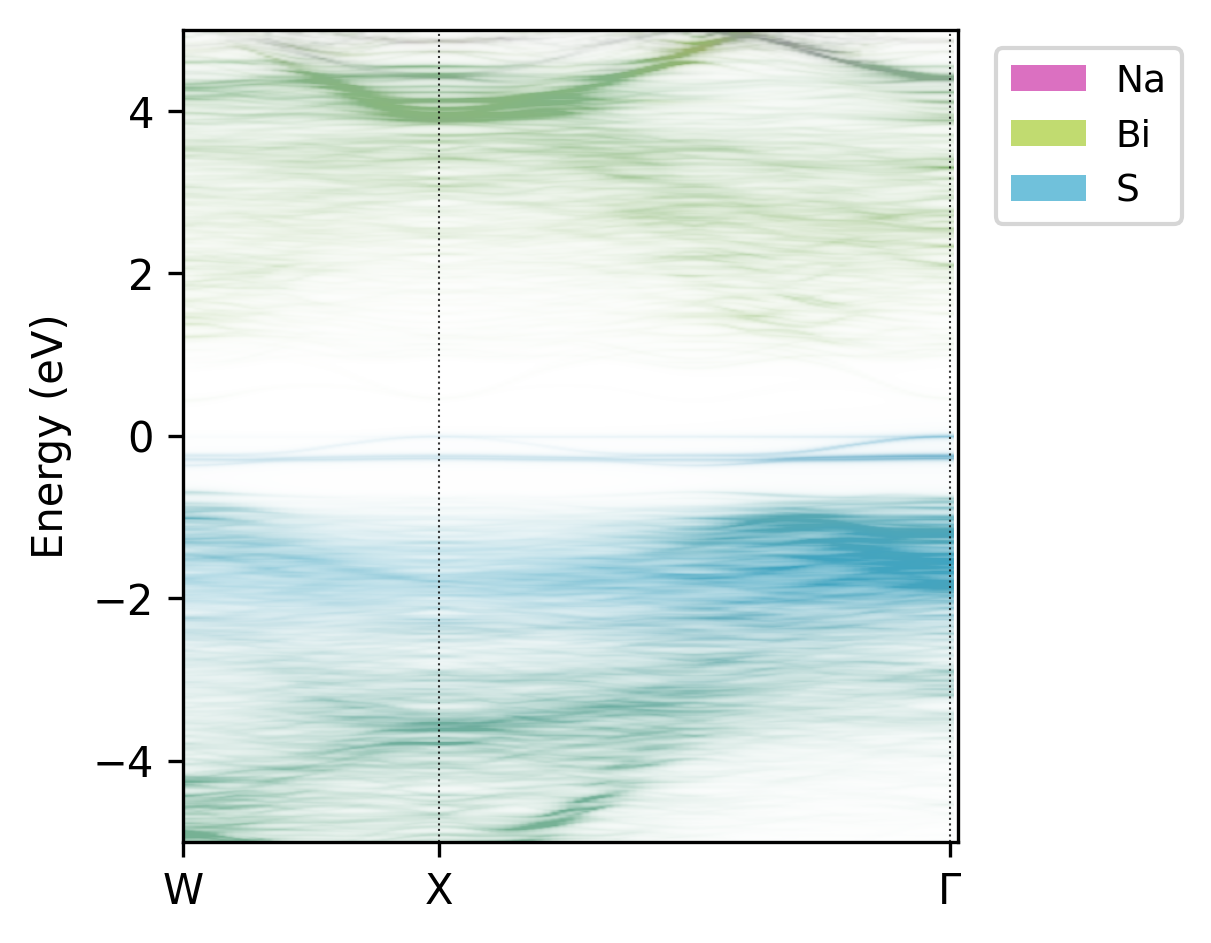
Unfolded band structure of NaBiS2 with atomic contributions.#
Tip
If the k-points have been split into multiple calculations (e.g. hybrid DFT band structures), the --procar option
should be passed multiple times to specify the path to each split PROCAR(.gz) file (i.e.
--procar calc1/PROCAR --procar calc2/PROCAR ...).
From this plot, we can see that sulfur anions dominate the valence band, while bismuth cations dominate the conduction band, with minimal contributions from the sodium cations as expected.
Note
The atomic projections are not stored in the easyunfold.json data file, so the PROCAR(.gz) file
should be kept for replotting in the future.
While the main conclusions of S dominating the valence band and Bi dominating the conduction band are clear from the plot above, the high intensity of the S projections in the valence band makes the Bi contributions in the conduction band more faint and less apparent.
So, we can create separated plots for each atom type to make their individual contributions more clear, by omitting the
--combined tag:
easyunfold unfold plot-projections --atoms="Na,Bi,S" --cmap="bone_r" --intensity 2
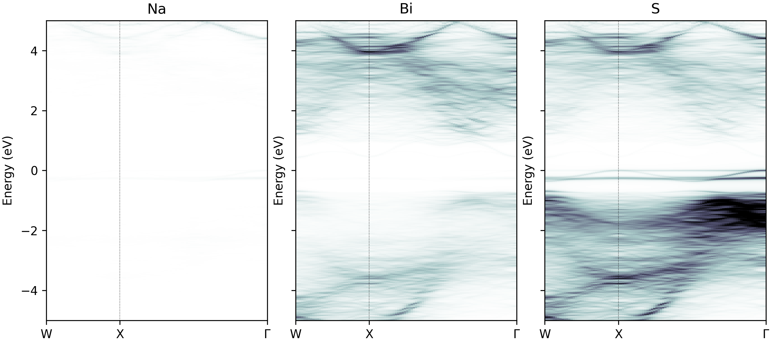
Unfolded band structure of NaBiS2 with atomic contributions plotted separately.#
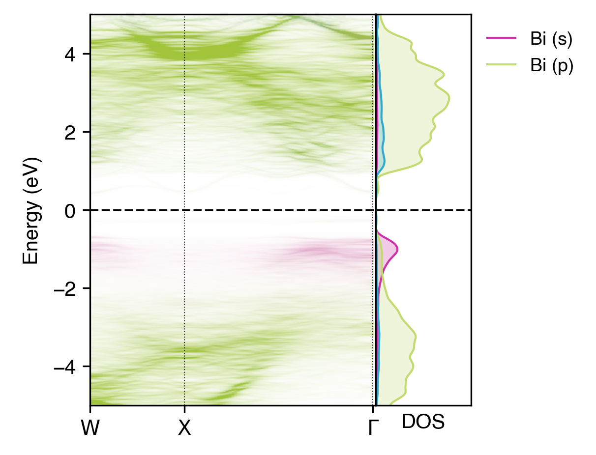
An alternative option here is also to just plot only the contributions of Na and Bi cations, with no S projections:
easyunfold unfold plot-projections --atoms="Na,Bi" --intensity 3 --combined
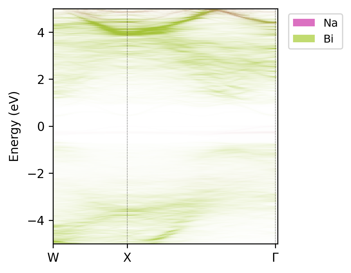
Unfolded band structure of NaBiS2 with atomic contributions of only Na and Bi.#
While this plot isn’t the most aesthetic, it clearly shows that Bi (green) contributes to both the conduction band and (less so) valence band states, but Na (red) doesn’t contribute significantly at or near the band edges (it’s a spectator ion!).
Atom-projected Unfolded Band Structure with DOS#
We can also combine the atom projections with the DOS plotting, using the --dos option as before:
easyunfold unfold plot-projections --atoms "Na,Bi,S" --intensity 3 --combined --dos vasprun.xml.gz --zero-line \
  --dos-label "DOS" --gaussian 0.1 --no-total --scale 2
Atom-projected unfolded band structure of NaBiS2 alongside the electronic density of states (DOS)#
The orbital contributions of elements in the DOS plot are automatically coloured to match that of the atomic
projections in the unfolded band structure plot, and these colours can be changed with the --colours option (as shown
in the MgO example).
Unfolded Band Structure with Specific Atom Selection#
In certain cases, we may want to project the contributions of specific atoms to the unfolded band structure, rather
than all atoms of a certain element. For example, in this example case of NaBiS\(_2\), we see that a flat localised state
is forming within the ‘bulk’ band gap. We can show that this state is contributed by only one or two atoms in the
supercell, using the --atoms-idx option:
easyunfold unfold plot-projections -unfold plot-projections --atoms-idx="1-55,57-65,67-80|56,66" --intensity 2
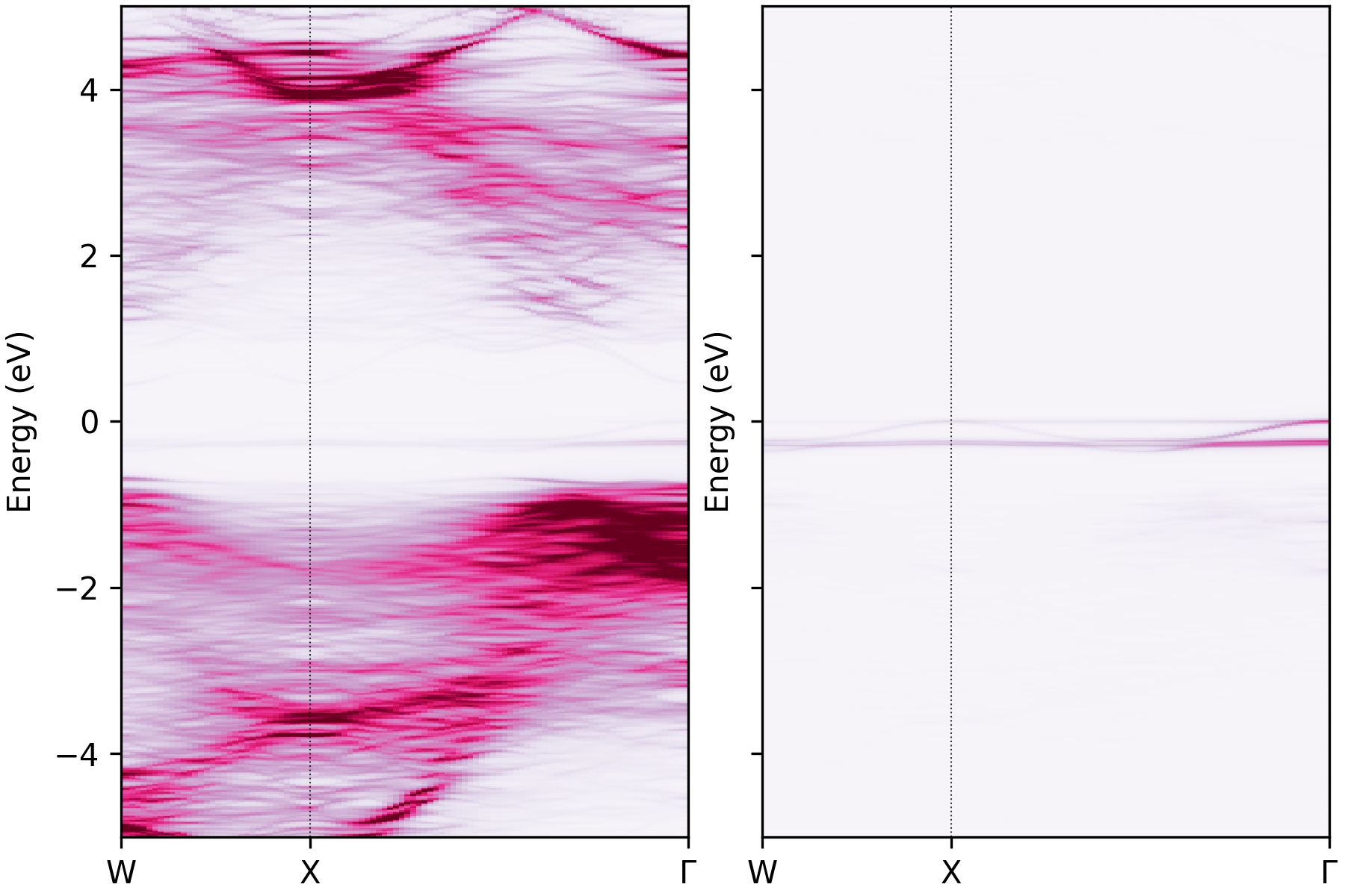
Unfolded band structure of NaBiS2 with the atomic contributions of atoms 56 and 66 plotted separately.#
Here we can see that this in-gap localised state is dominated by only two (sulfur) atoms in the supercell (atoms 56
and 66), which correspond to Na-rich pockets in NaBiS2, as discussed in Huang & Kavanagh et al. [1].
Note
The --atoms-idx option is used to specify the atoms to be projected onto the unfolded band structure. This takes a
string of the form a-b|c-d|e-f where a, b, c, d, e and f are integers corresponding to the atom indices
in the VASP structure file (i.e. POSCAR/CONTCAR, corresponding to the PROCAR(.gz) being used to obtain the
projections). Different groups are separated by |, and - can be used to define the range for each projected atom
type. A comma-separated list can also be used instead of ranges with hyphens. Note that 1-based indexing is used for
atoms, matching the convention in VASP, which is then converted to zero-based indexing internally in python.
Unfolded Band Structure with Orbital Projections#
If we want to see the contributions of specific orbitals to the unfolded band structure, we can use the --orbitals
option. This takes a string of the form a,b|c|d,e,f where a, b, c, d, e and f are the orbitals we want
to project onto the unfolded band structure.
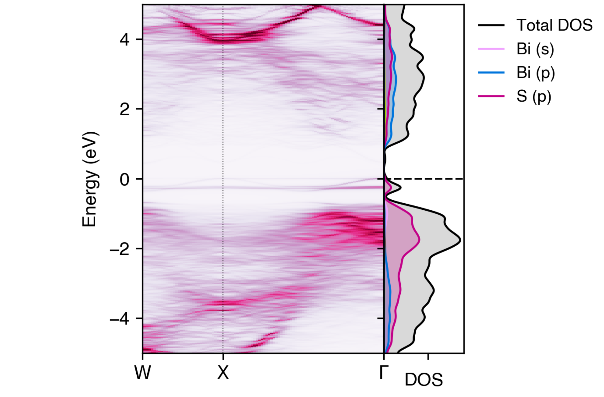
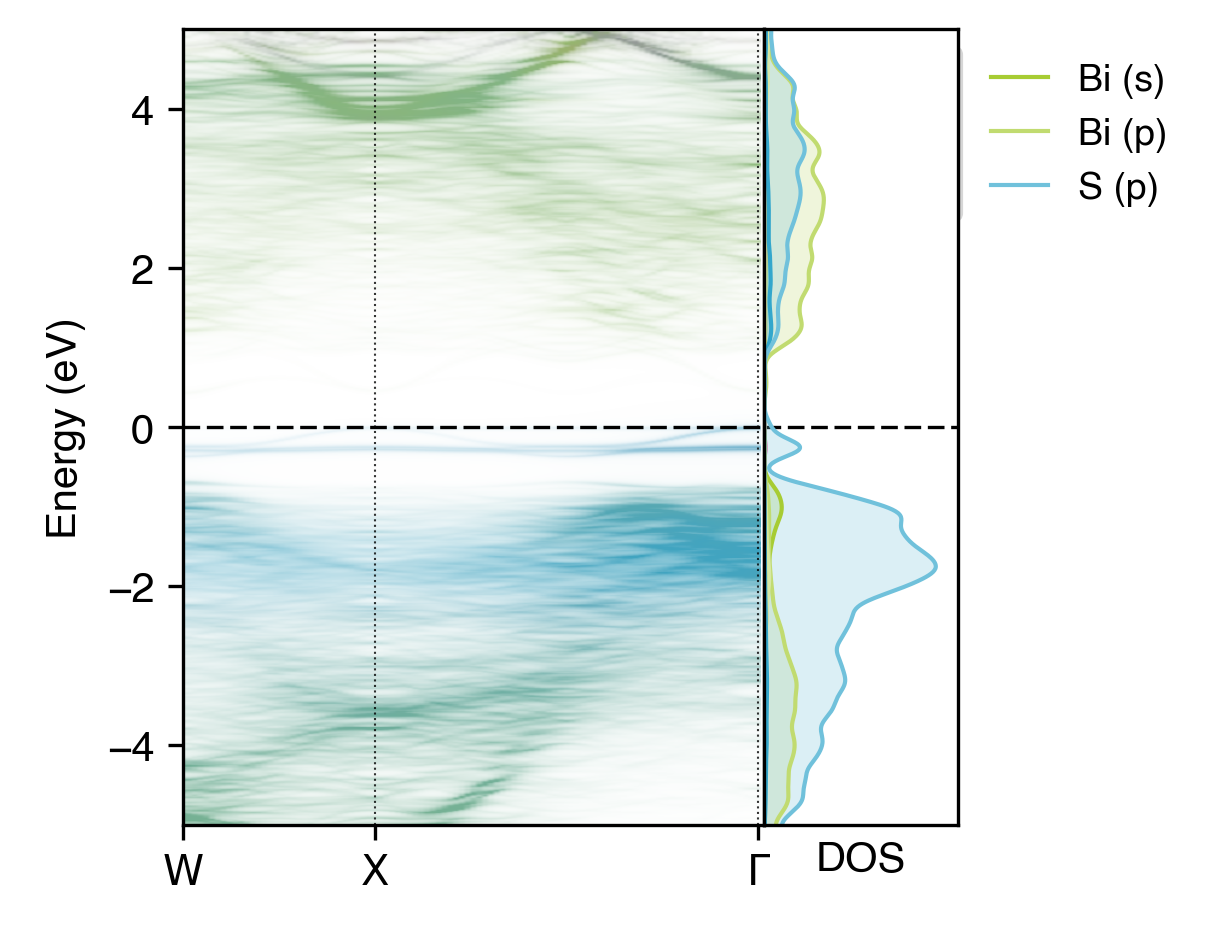
For example, if we want to see the contributions of the Bi \(s\), \(p\) and S \(s\) orbitals to the unfolded band structure, we can use the following command:
easyunfold unfold plot-projections --atoms "Bi,Bi,S" --orbitals="s|p|s"  --intensity 3  --combined \
  --dos vasprun.xml.gz --zero-line --dos-label "DOS" --gaussian 0.1 --no-total --scale 5
Orbital-projected unfolded band structure of NaBiS2 alongside the electronic density of states (DOS)#
Here we have separated out the contributions of Bi \(s\) orbitals (which have some weak anti-bonding contributions to the upper ‘bulk’ VBM as expected, due to the occupied Bi lone-pair; see refs [1] and [2]) and \(p\) orbitals (which contribute to the conduction band and lower valence band). We have also shown only the \(s\) orbital contributions of sulfur, which we can see have minimal contributions to the electronic structure near the band gap.
\(lm\)-decomposed Orbital Projections#
We can also use the --orbitals option to project onto specific \(lm\)-decomposed orbitals, and/or use the
--dos-orbitals option to split the DOS plot into \(lm\)-decomposed orbital contributions. For example, if we want to
see the contributions of the Bi and S \(p_x\), \(p_y\) and \(p_z\) orbitals to the unfolded band structure, we can use the
following command:
easyunfold unfold plot-projections --atoms "Na,Bi,S" --orbitals="all|px,py,pz|px,py,pz" --intensity 3 --combined \
  --dos vasprun.xml.gz --zero-line --dos-label "DOS" --gaussian 0.1 --no-total --scale 6
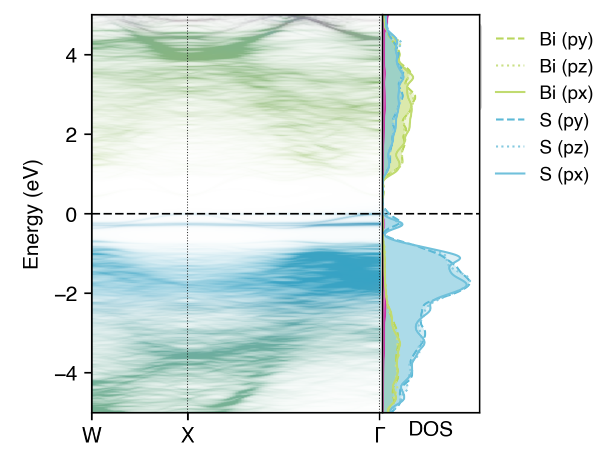
\(lm\)-decomposed orbital-projected unfolded band structure of NaBiS2 alongside the DOS#
Here, the \(p_x\), \(p_y\) and \(p_z\) orbitals do not differ significantly in their contributions to the electronic structure, due to the cubic symmetry of the NaBiS2 crystal structure. However, in other cases, such as for the \(d\) orbitals of transition metals in octahedral/tetrahedral environments, we would expect to see significant differences in the contributions of different \(lm\)-decomposed orbitals to the electronic structure.
Tip
There are many customisation options available for the plotting functions in easyunfold. See easyunfold plot -h or
easyunfold unfold plot-projections -h for more details!