MgO with atomic projections, effective masses & defects#
Note
The files needed for this example are provided in the examples/MgO folder.
Often it is useful to know the various contributions of atoms in the structure to the electronic bands in the band structure, to analyse the chemistry and orbital interactions at play in the system. This can be computed for unfolded bands as well.
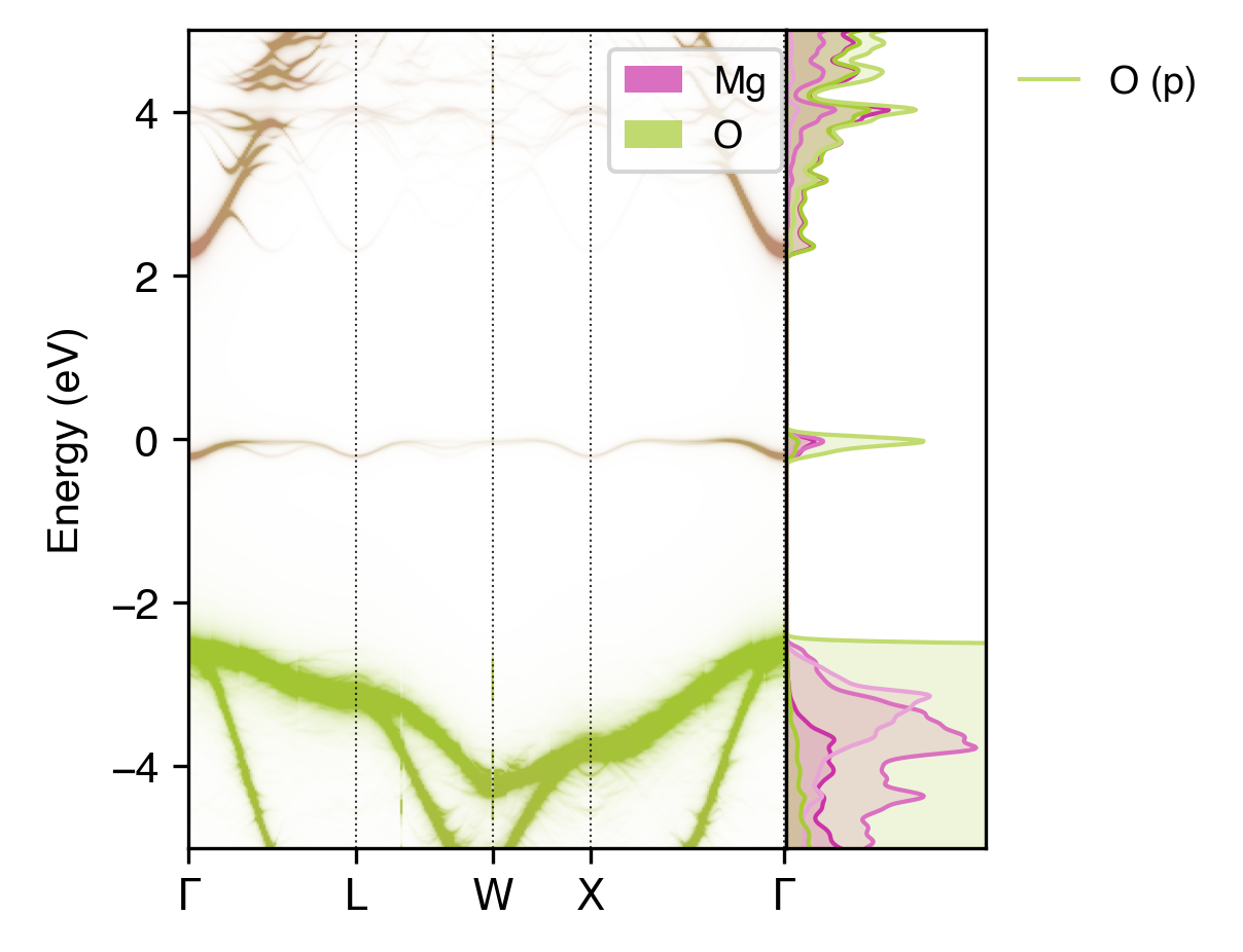
For a normal band structure calculation, the contributions can be inferred by colouring the band according to the elemental contributions, which can be done using sumo.
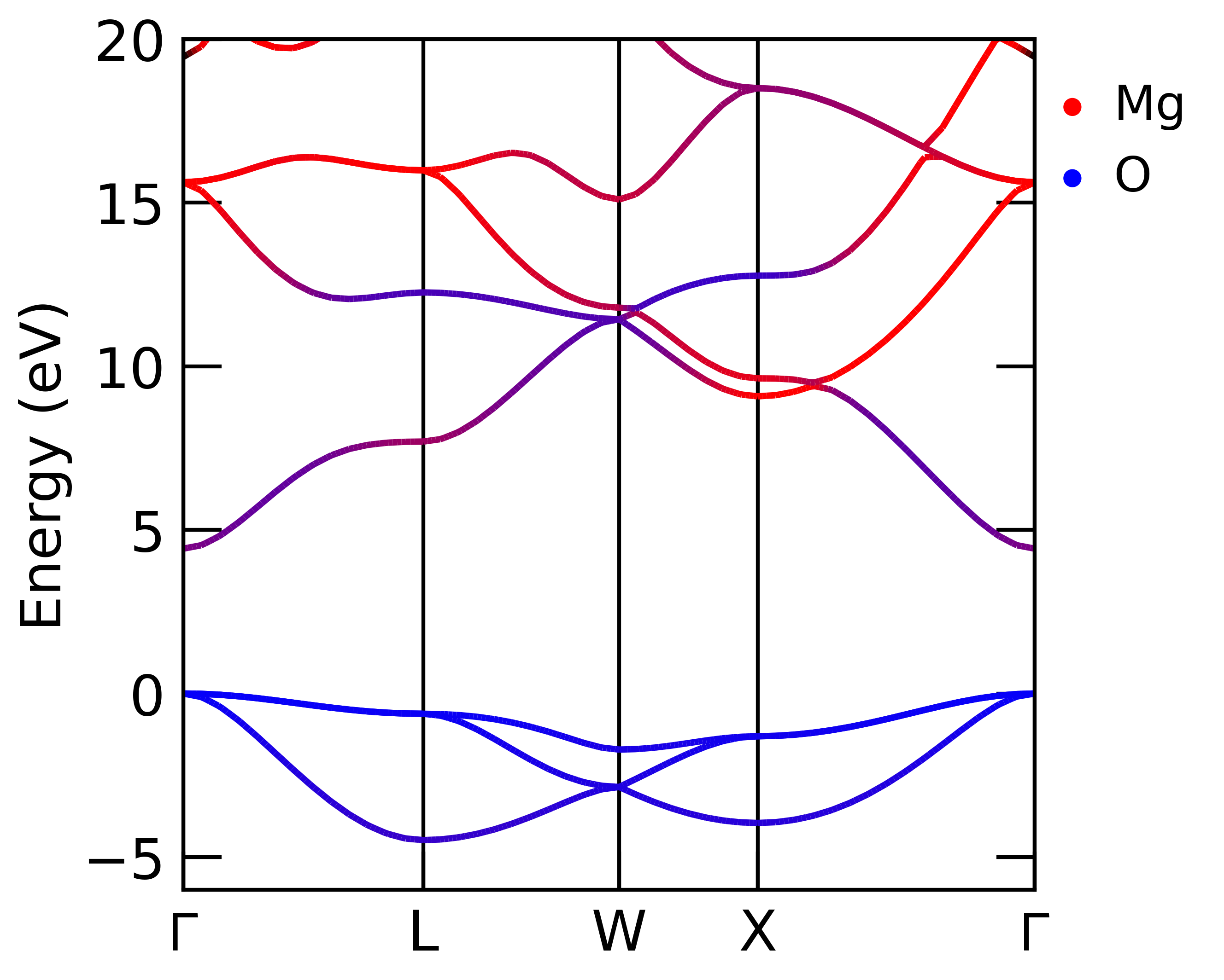
Band structure of MgO with atomic contribution
Similar plots can be generated for unfolded band structures. However, because the unfolded spectral function itself contains both the location of the band and its intensity, adding a third dimension of information (atomic projection) can be tricky to visualise.
Displaced Mg Supercell Band Unfolding#
In this example, we unfold the bands from a MgO 2x1x2 supercell with a Mg atom displaced to break symmetry. The procedure is essentially the same as described in the Si supercell example.
The only difference here is that we turn on the calculation of orbital projections in VASP with
LORBIT = 11 (12, 13 and 14 will also work) in the INCAR file, and then use the plot-projections subcommand
when plotting the unfolded band structure:
easyunfold unfold plot-projections --procar MgO_super/PROCAR.gz --atoms="Mg,O" --combined --emin=-6 \
--emax=20 --intensity 6.5 --poscar MgO_super/POSCAR
Note that the path of the PROCAR(.gz) is passed along with the desired atom projections (Mg and O here).
Tip
If the k-points have been split into multiple calculations (e.g. hybrid DFT band structures), the --procar option
should be passed multiple times to specify the path to each split PROCAR(.gz) file (i.e.
--procar calc1/PROCAR --procar calc2/PROCAR ...).
Note
The atomic projections are not stored in the easyunfold.json data file, so the PROCAR(.gz) file(s)
should be kept for replotting in the future.
The --combined option creates a combined plot with different colour maps for each atomic grouping.
The spectral intensity is used to define the transparency (alpha) allowing the fusion of multiple
projections into a single plot.
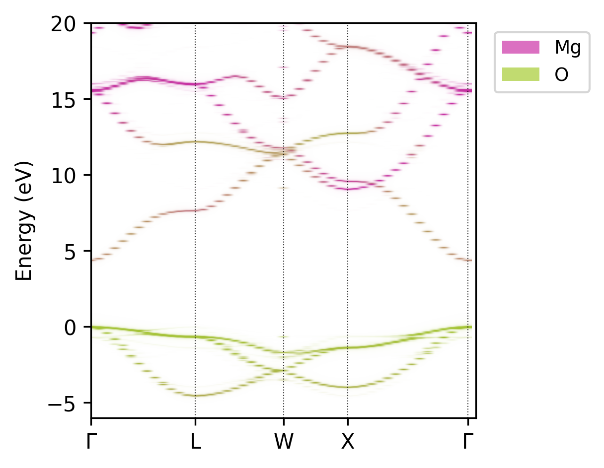
Unfolded MgO band structure with atomic projections.#
The default colour map for atom projections is red, green, blue and purple for the 1st, 2nd, 3rd and 4th atomic species
specified. This can be changed with the --colours option, as well as several other plotting/visualisation settings –
see the output of easyunfold unfold plot-projections --help for more details. If we wanted to plot the atomic
projections with the same colouring scheme as the sumo plot above (i.e. red for Mg and blue for O), we can use:
easyunfold unfold plot-projections --procar MgO_super/PROCAR --atoms="Mg,O" --combined --emin=-6 \
--emax=20 --intensity 6.5 --colours "r,b"
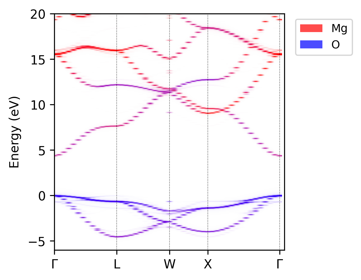
Unfolded MgO band structure with atomic projections; red for Mg and blue for O atoms.#
Note
In order to specify the atomic projections with --atoms, the POSCAR or CONTCAR file for the supercell must be
present. If this is not the case, or we want to use projections from only specific atom subsets in the supercell, we can
alternatively use the --atoms-idx tag. This takes a string of the form a-b|c-d|e-f where a, b, c, d, e and
f are integers corresponding to the atom indices in the VASP structure file (i.e. POSCAR/CONTCAR, corresponding
to the PROCAR(.gz) being used to obtain the projections). Different groups are separated by |, and -
can be used to define the range for each projected atom type. A comma-separated list can also be used instead of ranges
with hyphens. Note that 1-based indexing is used for atoms, matching the convention in VASP, which is then converted to
zero-based indexing internally in python. In this example, we could set --atoms-idx="1-4|5-8" to get the same result
as --atoms="Mg,O" (but without the figure legend).
In some cases, especially if there are many projection to be plotted at the same time, it can be clearer to create
separated plots for each. This is the default behaviour for plot-projections, when --combined is not specified.
easyunfold unfold plot-projections --procar MgO_super/PROCAR --atoms="Mg,O" --emin=-6 \
--emax=20 --intensity 6.5
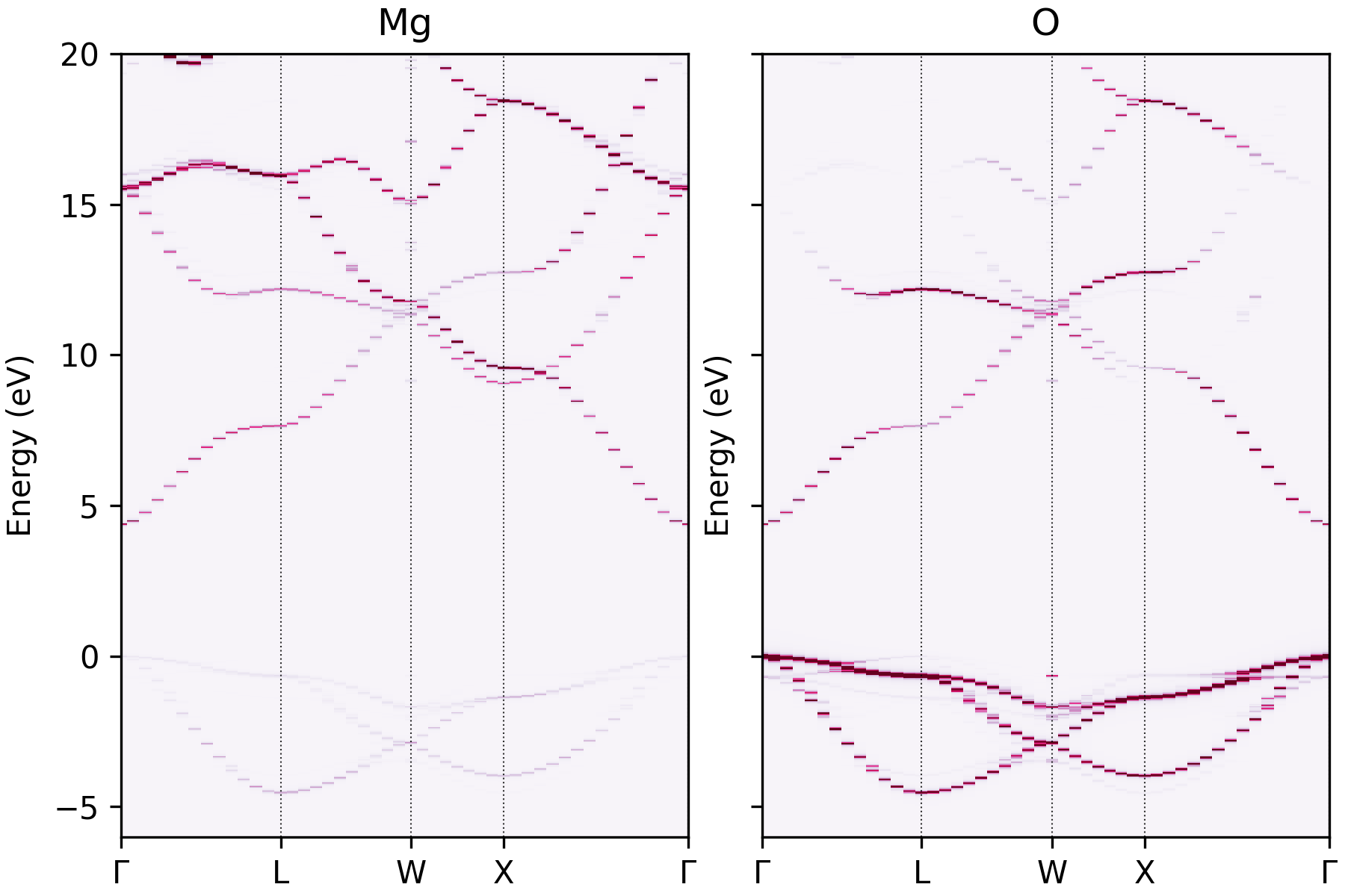
Unfolded MgO band structure with atomic projections plotted separately.#
Tip
There are many customisation options available for the plotting functions in easyunfold. See easyunfold plot -h or
easyunfold unfold plot-projections -h for more details!
Warning
If your PROCAR(.gz) file(s) are corrupted or incomplete, the plot-projections command will fail with an error message like ValueError: cannot reshape array of size 73542192 into shape (2,74,348,90,16). In cases where the start/end of the PROCAR file looks fine, this can sometimes be checked with grep -E '[^[:print:]]' --color=never PROCAR which will only show an output if some lines in the file are corrupted. Typically this requires re-running the VASP calculation to give an uncorrupted file.
Carrier Effective Masses#
The command easyunfold unfold effective-mass can be used to find the effective masses of the unfolded band structure.
The example output is shown below:
Loaded data from easyunfold.json
Band extrema data:
  Kpoint index  Kind      Sub-kpoint index    Band indices
--------------  ------  ------------------  --------------
             0  cbm                      0              16
            47  cbm                      0              16
             0  vbm                      0              15
            47  vbm                      0              15

Electron effective masses:
  index  Kind      Effective mass    Band index  from                      to
-------  ------  ----------------  ------------  ------------------------  -------------------
      0  m_e             0.373553            16  [0.0, 0.0, 0.0] (\Gamma)  [0.5, 0.5, 0.5] (L)
      1  m_e             0.367203            16  [0.0, 0.0, 0.0] (\Gamma)  [0.5, 0.0, 0.5] (X)

Hole effective masses:
  index  Kind      Effective mass    Band index  from                      to
-------  ------  ----------------  ------------  ------------------------  -------------------
      0  m_h             -3.44604            15  [0.0, 0.0, 0.0] (\Gamma)  [0.5, 0.5, 0.5] (L)
      1  m_h             -2.13525            15  [0.0, 0.0, 0.0] (\Gamma)  [0.5, 0.0, 0.5] (X)
Unfolded band structure can be ambiguous, please cross-check with the spectral function plot.
If detected band extrema are not consistent with the band structure, or some band edges are not detected, one should adjust the --intensity-threshold and --extrema-detect-tol.
Increasing the value of --intensity-threshold will filter away bands with very small spectral weights.
On the other hand, increasing --extrema-detect-tol will increase the energy window with respect
to the VBM or CBM to assign extrema points.
One can also inspect if the detected bands makes sense by using the --plot or --plot-fit options, in which case it can be useful to increase --npoints to extend the plotted range.
A Jupyter Notebook example can be found here.
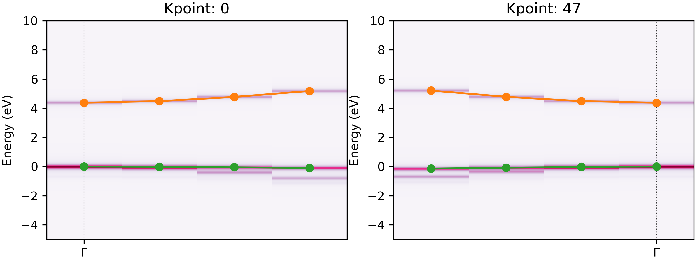
Extracted bands at CBM and VBM for an unfolded MgO band structure.#
Warning
Make sure the band extrema data tabulated is correct and consistent before using any of the reported values. The results can unreliable for systems with little or no band gaps and those with complex unfolded band structures.
Tip
For complex systems where the detection is difficult, one can manually pass the kpoint and the band indices using the --manual-extrema option, or can pass the eigenvalue of the band edge of interest using the --extremum-eigenvalue option. See easyunfold unfold effective-mass -h for more details.
Defects#
As shown in the easyunfold YouTube tutorial, band structure unfolding can often be useful for analysing the impact of defects and dopants on the electronic structure of materials – particularly under high concentrations.
As a brief example, here we show base steps in calculating the unfolded band structure of a defective supercell with easyunfold, following the procedure shown in the YouTube tutorial.
Step 1. Defect Supercell Generation#
For this, we can use the doped defect package as shown in the tutorial:
from pymatgen.core.structure import Structure
from doped.generation import DefectsGenerator

mgo_prim = Structure.from_file('MgO_prim_POSCAR')
defect_gen = DefectsGenerator(mgo_prim)
Generating DefectEntry objects: 100.0%|██████████| [00:23,   4.26it/s]
Vacancies    Guessed Charges    Conv. Cell Coords    Wyckoff
-----------  -----------------  -------------------  ---------
v_Mg         [+1,0,-1,-2]       [0.000,0.000,0.000]  4a
v_O          [+2,+1,0,-1]       [0.500,0.500,0.500]  4b

Substitutions    Guessed Charges    Conv. Cell Coords    Wyckoff
---------------  -----------------  -------------------  ---------
Mg_O             [+4,+3,+2,+1,0]    [0.500,0.500,0.500]  4b
O_Mg             [0,-1,-2,-3,-4]    [0.000,0.000,0.000]  4a

Interstitials    Guessed Charges    Conv. Cell Coords    Wyckoff
---------------  -----------------  -------------------  ---------
Mg_i_Td          [+2,+1,0]          [0.250,0.250,0.250]  8c
O_i_Td           [0,-1,-2]          [0.250,0.250,0.250]  8c

The number in the Wyckoff label is the site multiplicity/degeneracy of that defect in the conventional ('conv.') unit cell, which comprises 4 formula unit(s) of MgO.
Note that Wyckoff letters can depend on the ordering of elements in the conventional standard structure, for which doped uses the spglib convention.
and then write the VASP output files for the supercell relaxations:
from doped.vasp import DefectsSet

ds = DefectsSet(defect_gen)
ds.write_files(unperturbed_poscar=True)  # skipping structure-searching for this example
Step 2. Band Structure k-point Generation#
When our defect supercell relaxations have completed, we can then generate our k-point paths for the supercell band structure calculation, as usual with easyunfold:
easyunfold generate MgO_prim_POSCAR supercell_POSCAR MgO_prim_KPOINTS_band --scf-kpoints supercell_IBZKPT
where MgO_prim_KPOINTS_band contains the k-point path for the primitive cell band structure (e.g. generated by sumo-kgen) and here we are performing a hybrid DFT calculation and so we need to use the --scf-kpoints option. If for any reason easyunfold cannot automatically guess the supercell transformation matrix, we can also access this from the doped DefectsGenerator.supercell_matrix attribute and supply this with the --matrix option.
Step 3. Band Structure Parsing#
When our supercell band structure calculation has then completed, we can parse the wavefunction output to obtain the unfolded band structure:
easyunfold unfold calculate WAVECAR
and then plot the unfolded band structure with atomic projections:
easyunfold unfold plot-projections --intensity 60 --dos vasprun.xml.gz --gaussian 0.03 --atoms="Mg,O" --combined --scale 40 --no-total
Atom-projected unfolded band structure for a neutral oxygen vacancy in MgO, showing that the single-particle state introduced by the vacancy is the band gap is comprised of both Mg and O contributions.#
Note
The example files for this unfolded band structure calculation of the neutral oxygen vacancy supercell are provided in the examples/MgO/v_O_0_YT_tutorial folder.